import numpy as np
import matplotlib.pyplot as plt

# plt.style.use('fivethirtyeight')
import pandas as pd
import statsmodels.api as sm
import pymc as pm
WARNING (pytensor.tensor.blas): Using NumPy C-API based implementation for BLAS functions.import numpy as np
import matplotlib.pyplot as plt
# plt.style.use('fivethirtyeight')
import pandas as pd
import statsmodels.api as sm
import pymc as pmWARNING (pytensor.tensor.blas): Using NumPy C-API based implementation for BLAS functions.The generalized linear model (GLM) is simply an umbrella term for all linear models which are not simple/multiple linear regression models, in econometrics we have seen logit, probit, tobit and etc., they are all generalized linear models.
As a reminder, the linear regression model’s predicted values take the form \[ \hat{Y}=X\beta \] To formulate a generalized linear model, we impose an arbitrary function onto the linear combination, i.e. \[ \tilde{Y} = f(X\beta) \] where \(f\) is called the inverse link function.
The most famous type of GLM is logistic regression which is also called logit regression in the context of econometrics. Here we provide a brief refresh of logit regression.
A simple logit model hypothesizes a sigmoid shape function \[ P_i = \frac{1}{1+e^{-(\beta_1+\beta_2X_i)}} \] where the inverse link function is \(\frac{1}{1+e^{-z}}\), and \(z\) represents the predicted value of a linear model.
z = np.linspace(-8, 8)
fig, ax = plt.subplots(figsize=(8, 5))
ax.plot(z, 1 / (1 + np.exp(-z)))
ax.set_xlabel("z")
ax.set_ylabel(r"$P = 1/(1+e^{-Z})$")
ax.grid()
plt.show()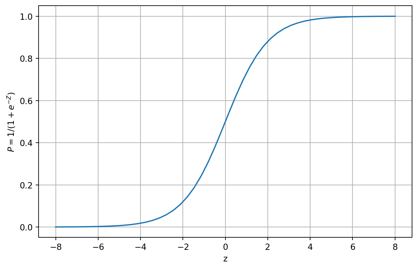
No matter what value we receive from \(z\) (infinite domain), the final result will be transformed into a \([0, 1]\) range. The
We usually denote \(Z_i = \beta_1+\beta_2X_i\), ranges from $(-, +) $. This model solves the issues of probabilistic range and linear model.
In order to estimate the logit model, we are seeking ways to linearize it. It might look confusing at first sight, here is the steps \[ P_{i}=\frac{1}{1+e^{-Z_{i}}}=\frac{e^{Z_i}}{e^{Z_i}}\frac{1}{1+\frac{1}{e^{Z_i}}}=\frac{e^{Z_i}}{1+e^{Z_i}} \]
And \(1-P_i\) \[ 1-P_{i}=\frac{1}{1+e^{Z_{i}}} \]
Combine them, we have the odds ratios \[ \frac{P_{i}}{1-P_{i}}=\frac{1+e^{Z_{i}}}{1+e^{-Z_{i}}}=e^{Z_{i}} \]
Here’s the interesting part, take natural log, we get a linearized model and we commonly call the log odds ratios the logit. \[ \underbrace{\ln{\bigg(\frac{P_{i}}{1-P_{i}}\bigg)}}_{\text{logit}}= Z_i =\beta_1+\beta_2X_i \]
To estimate the model, some technical procedures have to be carried out. Logit wouldn’t have any meaningful interpretation, if we simply plug in the data \(Y_i\). Because we don’t observe \(P_i\), the results are nonsensical. \[ \ln \left(\frac{1}{0}\right) \quad \text{if a family own a house}\\ \ln \left(\frac{0}{1}\right) \quad \text{if a family does not own a house} \]
One way to circumvent this technical issue, the data can be grouped to compute \[ \hat{P}_{i}=\frac{n_{i}}{N_{i}} \] where \(N_i\) is number of families in a certain income level, e.g. \([20000, 29999]\), and \(n_i\) is the number of family owning a house in the that level.
However, this is not a preferred method, since we have nonlinear tools here. Recall that owning a house is following a Bernoulli distribution whose probability mass function is \[ f_i(Y_i)= P_i^{Y_i}(1-P_i)^{1-Y_i} \] The joint distribution is the product of Bernoulli PMF due to their independence \[ f\left(Y_{1}, Y_{2}, \ldots, Y_{n}\right)=\prod_{i=1}^{n} f_{i}\left(Y_{i}\right)=\prod_{i=1}^{n} P_{i}^{Y_{i}}\left(1-P_{i}\right)^{1-Y_{i}} \]
In order to obtain log likelihood function, we take natural log \[ \begin{aligned} \ln f\left(Y_{1}, Y_{2}, \ldots, Y_{n}\right) &=\sum_{i=1}^{n}\left[Y_{i} \ln P_{i}+\left(1-Y_{i}\right) \ln \left(1-P_{i}\right)\right] \\ &=\sum_{i=1}^{n}\left[Y_{i} \ln P_{i}-Y_{i} \ln \left(1-P_{i}\right)+\ln \left(1-P_{i}\right)\right] \\ &=\sum_{i=1}^{n}\left[Y_{i} \ln \left(\frac{P_{i}}{1-P_{i}}\right)\right]+\sum_{i=1}^{n} \ln \left(1-P_{i}\right) \end{aligned} \] Replace \[ \ln{\bigg(\frac{P_{i}}{1-P_{i}}\bigg)}=\beta_1+\beta_2X_i\\ 1-P_{i}=\frac{1}{1+e^{\beta_1+\beta_2X_i}} \]
Finally we have log likelihood function of \(\beta\) \[ \ln f\left(Y_{1}, Y_{2}, \ldots, Y_{n}\right)=\sum_{i=1}^{n} Y_{i}\left(\beta_{1}+\beta_{2} X_{i}\right)-\sum_{i=1}^{n} \ln \left[1+e^{\left(\beta_{1}+\beta_{2} X_{i}\right)}\right] \] Take partial derivative w.r.t to \(\beta_2\) \[ \frac{\partial LF}{\partial \beta_2} = n\beta_2 -\sum_{i=1}^n\frac{e^{\beta_1+\beta_2X_i}X_i}{1+e^{\beta_1+\beta_2X_i}}=0 \] And stop here, apparently there won’t be analytical solutions, i.e. numerical solutions are necessary. And this is exactly what Python is doing for us below.
Here we come back to the apartment owning example. The data is an excerpt of survey of citizens in Manchester, UK.
df = pd.read_excel(
    "Basic_Econometrics_practice_data.xlsx", sheet_name="HouseOwn_Quali_Resp"
)
df.head()

Y = df[["Own_House"]]
X = df[["Annual_Family_Income"]]
X = sm.add_constant(X)

log_reg = sm.Logit(Y, X).fit()
Optimization terminated successfully.
Current function value: 0.257124
Iterations 8Optimization of likelihood function is an iterative process and global optimization has been reached as the notice shows.
Print the estimation results.
print(log_reg.summary()) Logit Regression Results
==============================================================================
Dep. Variable: Own_House No. Observations: 38
Model: Logit Df Residuals: 36
Method: MLE Df Model: 1
Date: Fri, 13 Sep 2024 Pseudo R-squ.: 0.6261
Time: 08:59:00 Log-Likelihood: -9.7707
converged: True LL-Null: -26.129
Covariance Type: nonrobust LLR p-value: 1.067e-08
========================================================================================
coef std err z P>|z| [0.025 0.975]
----------------------------------------------------------------------------------------
const -6.7617 2.189 -3.088 0.002 -11.053 -2.471
Annual_Family_Income 0.1678 0.053 3.176 0.001 0.064 0.271
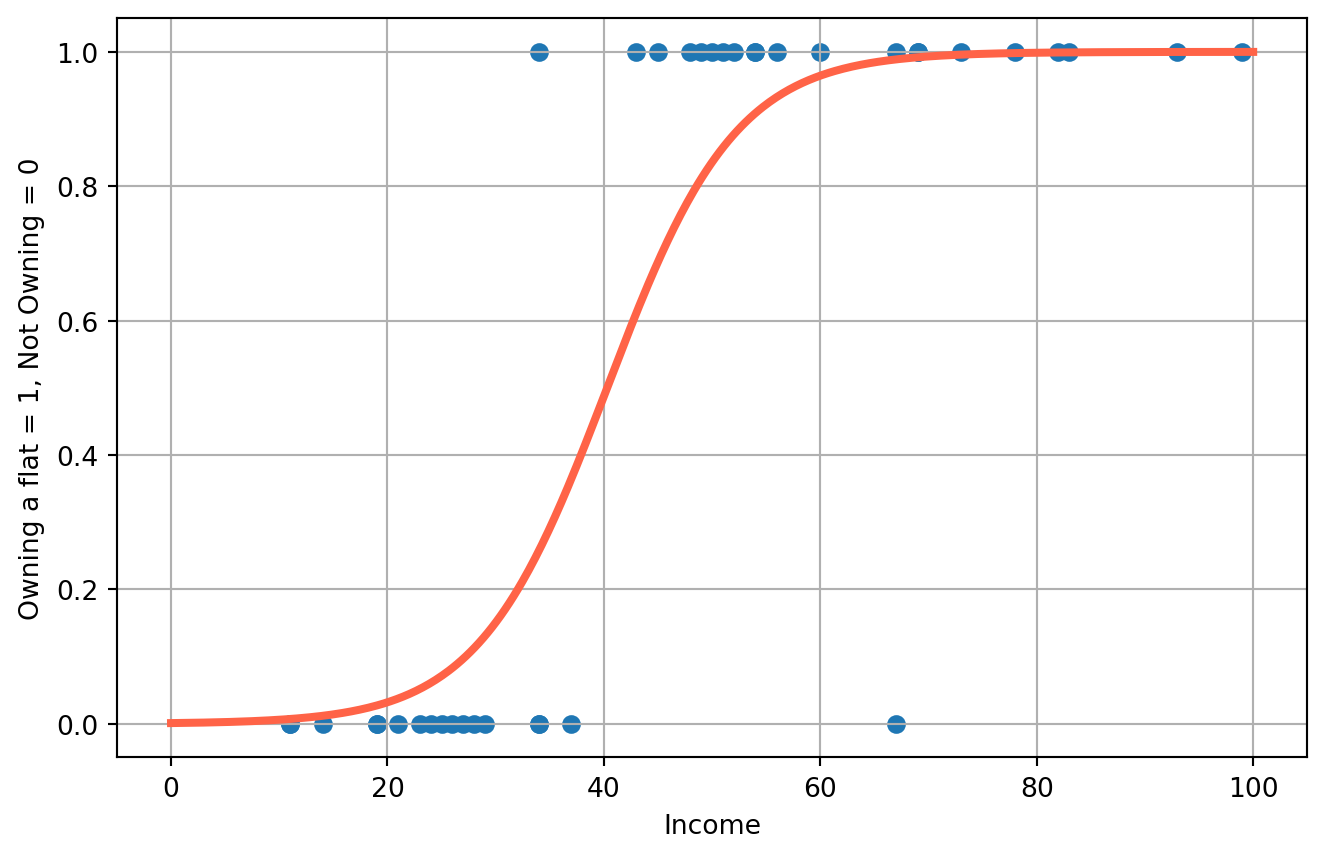
========================================================================================Here is the estimated model \[ \hat{P_i} = \frac{1}{1+e^{6.7617-0.1678 X_i}} \] And the fitted curve
X = np.linspace(0, 100, 500)
P_hat = 1 / (1 + np.exp(-log_reg.params[0] - log_reg.params[1] * X))

fig, ax = plt.subplots(figsize=(8, 5))
ax.scatter(df["Annual_Family_Income"], df["Own_House"])
ax.plot(X, P_hat, color="tomato", lw=3)
ax.set_xlabel("Income")
ax.set_ylabel("Owning a flat = 1, Not Owning = 0")
ax.grid()
plt.show()
/tmp/ipykernel_3706/2566141605.py:2: FutureWarning:
Series.__getitem__ treating keys as positions is deprecated. In a future version, integer keys will always be treated as labels (consistent with DataFrame behavior). To access a value by position, use `ser.iloc[pos]`
To interpret estimated coefficients, we can calculate the marginal effect by taking derivative w.r.t certain \(\beta\), in this case \(\beta_2\). \[ \frac{dP_i}{d X_i} = \frac{dP_i}{dZ_i}\frac{dZ_i}{dX_i}=\frac{e^{-Z_i}}{(1+e^{-Z_i})^2}\beta_2 \] Plot both accumulative and marginal effects
beta1_hat, beta2_hat = log_reg.params[0], log_reg.params[1]
X = np.linspace(0, 100, 500)

Z = beta1_hat + beta2_hat * X
dPdX = np.exp(-Z) / (1 + np.exp(-Z)) ** 2 * beta2_hat

fig, ax1 = plt.subplots(figsize=(8, 5))
ax1.scatter(df["Annual_Family_Income"], df["Own_House"])
ax1.plot(X, P_hat, color="tomato", lw=3, label="Accumulative Effect")
ax1.legend(loc="center left")

ax2 = ax1.twinx()
ax2.plot(X, dPdX, lw=3, color="Gold", label="Marginal Effect")
ax2.legend(loc="center right")
ax2.set_title("Accumulative and Marginal Effect of Family Income on Owning a House")
ax2.grid()
plt.show()
/tmp/ipykernel_3706/2209732860.py:1: FutureWarning:
Series.__getitem__ treating keys as positions is deprecated. In a future version, integer keys will always be treated as labels (consistent with DataFrame behavior). To access a value by position, use `ser.iloc[pos]`
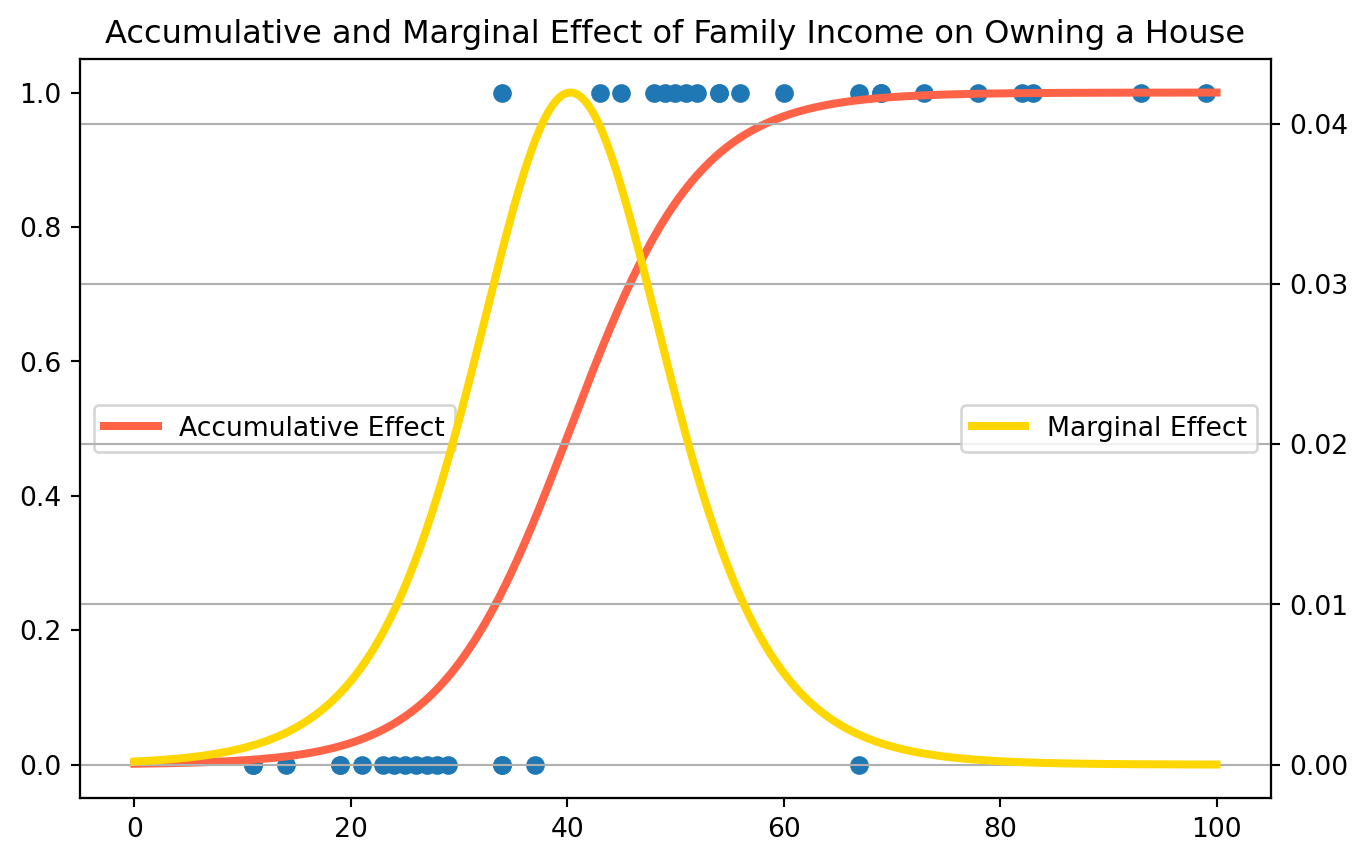
As family income raises, the marginal probability will reach maximum around \(40000\) pounds, to summarize the effect, we calculate the marginal effect at the mean value of the independent variables.
X_mean = np.mean(df["Annual_Family_Income"])
Z_mean_effect = beta1_hat + beta2_hat * X_mean
dPdX = np.exp(-Z_mean_effect) / (1 + np.exp(-Z_mean_effect)) ** 2 * beta2_hat
dPdX0.03297676614392625At the sample mean, \(1000\) pounds increase in family income increases the probability of owning a house by \(3.2 \%\).
with pm.Model() as model_0:
    beta1 = pm.Normal("beta1", mu=0, sigma=10)
    beta2 = pm.Normal("beta2", mu=0, sigma=10)

    mu = beta1 + beta2 * df["Annual_Family_Income"]
    theta = pm.Deterministic("theta", pm.math.sigmoid(mu))
    bd = pm.Deterministic("bd", -beta1 / beta2)

    yl = pm.Bernoulli("yl", p=theta, observed=df["Own_House"])

    trace_0 = pm.sample(1000, cores=1, return_inferencedata=True)
Auto-assigning NUTS sampler...
Initializing NUTS using jitter+adapt_diag...
Sequential sampling (2 chains in 1 job)
NUTS: [beta1, beta2]Sampling 2 chains for 1_000 tune and 1_000 draw iterations (2_000 + 2_000 draws total) took 7 seconds.
There were 3 divergences after tuning. Increase `target_accept` or reparameterize.
We recommend running at least 4 chains for robust computation of convergence diagnostics